Examples
Cortical Hemisphere
Here, we’ll perform an analysis similar to those included in our pre-print, using our example data.
First, create an instance of the Base class and generate 1000 surrogate maps:
from brainsmash.mapgen.base import Base
import numpy as np

# load parcellated structural neuroimaging maps
myelin = np.loadtxt("LeftParcelMyelin.txt")
thickness = np.loadtxt("LeftParcelThickness.txt")

# instantiate class and generate 1000 surrogates
gen = Base(myelin, "LeftParcelGeodesicDistmat.txt")  # note: can pass numpy arrays as well as filenames
surrogate_maps = gen(n=1000)
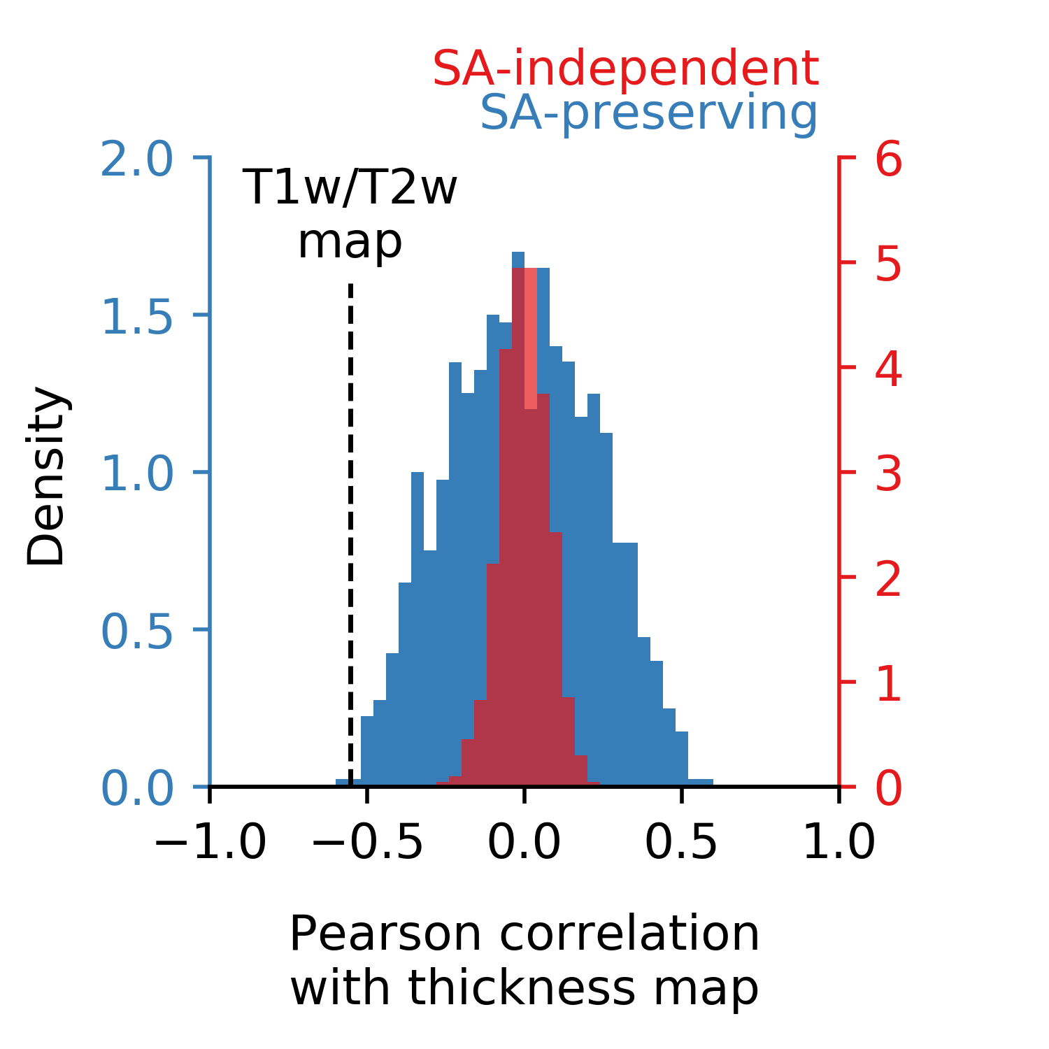
Next, compute the Pearson correlation between each surrogate myelin map and the empirical cortical thickness map:
from brainsmash.mapgen.stats import pearsonr, pairwise_r

surrogate_brainmap_corrs = pearsonr(thickness, surrogate_maps).flatten()
surrogate_pairwise_corrs = pairwise_r(surrogate_maps, flatten=True)
Repeat using randomly shuffled surrogate myelin maps:
naive_surrogates = np.array([np.random.permutation(myelin) for _ in range(1000)])
naive_brainmap_corrs = pearsonr(thickness, naive_surrogates).flatten()
naive_pairwise_corrs = pairwise_r(naive_surrogates, flatten=True)
Now plot the results:
import matplotlib.pyplot as plt
from scipy import stats

sac = '#377eb8'  # autocorr-preserving
rc = '#e41a1c'  # randomly shuffled
bins = np.linspace(-1, 1, 51)  # correlation b

# this is the empirical statistic we're creating a null distribution for
test_stat = stats.pearsonr(myelin, thickness)[0]

fig = plt.figure(figsize=(3, 3))
ax = fig.add_axes([0.2, 0.25, 0.6, 0.6])  # autocorr preserving
ax2 = ax.twinx()  # randomly shuffled

# plot the data
ax.axvline(test_stat, 0, 0.8, color='k', linestyle='dashed', lw=1)
ax.hist(surrogate_brainmap_corrs, bins=bins, color=sac, alpha=1,
    density=True, clip_on=False, zorder=1)
ax2.hist(naive_brainmap_corrs, bins=bins, color=rc, alpha=0.7,
    density=True, clip_on=False, zorder=2)

# make the plot nice...
ax.set_xticks(np.arange(-1, 1.1, 0.5))
ax.spines['left'].set_color(sac)
ax.tick_params(axis='y', colors=sac)
ax2.spines['right'].set_color(rc)
ax2.tick_params(axis='y', colors=rc)
ax.set_ylim(0, 2)
ax2.set_ylim(0, 6)
ax.set_xlim(-1, 1)
[s.set_visible(False) for s in [
    ax.spines['top'], ax.spines['right'], ax2.spines['top'], ax2.spines['left']]]
ax.text(0.97, 1.1, 'SA-independent', ha='right',va='bottom',
    color=rc, transform=ax.transAxes)
ax.text(0.97, 1.03, 'SA-preserving', ha='right', va='bottom',
    color=sac, transform=ax.transAxes)
ax.text(test_stat, 1.65, "T1w/T2w\nmap", ha='center', va='bottom')
ax.text(0.5, -0.2, "Pearson correlation\nwith thickness map",
    ha='center', va='top', transform=ax.transAxes)
ax.text(-0.3, 0.5, "Density", rotation=90, ha='left', va='center', transform=ax.transAxes)
plt.show()
Executing the above code produces the following figure:
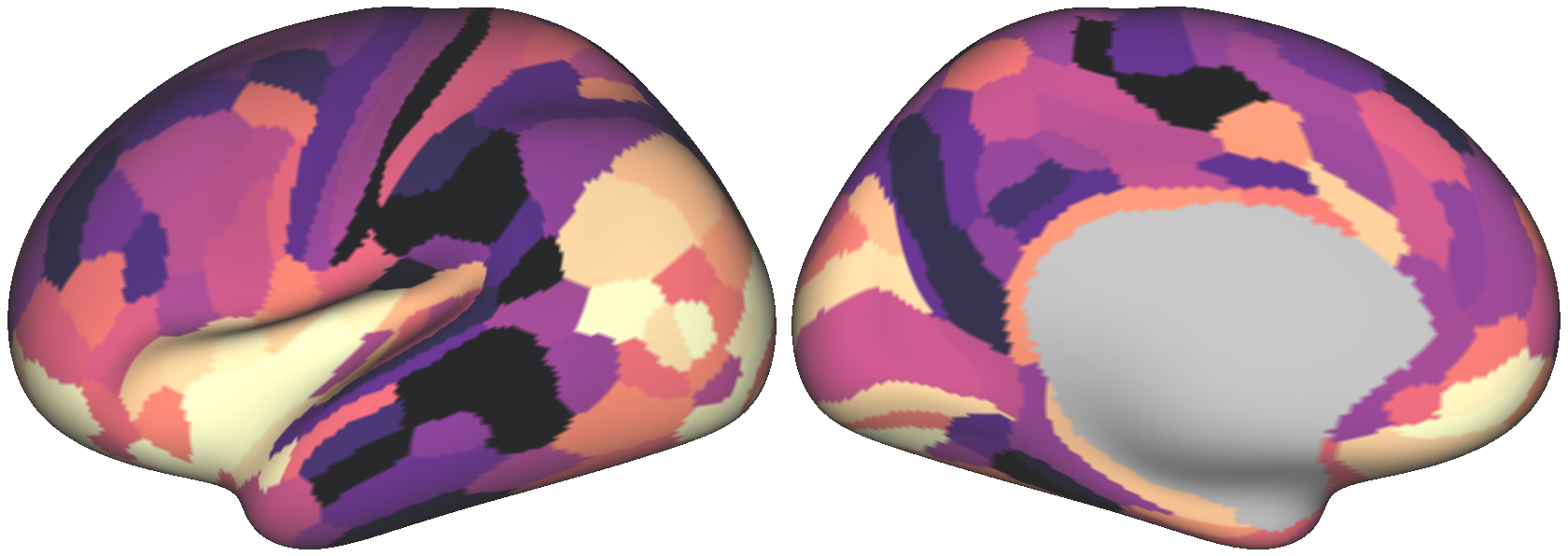
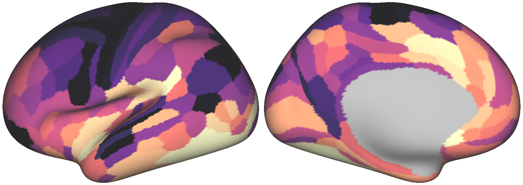
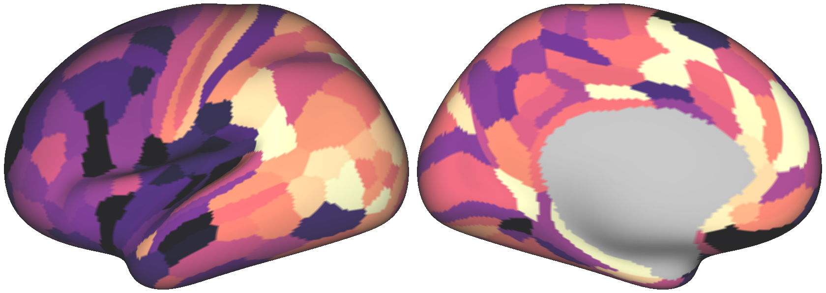
We can plot a couple surrogate maps on the cortical surface using wbplot:
from wbplot import pscalar

def vrange(x):
    return (np.percentile(x, 5), np.percentile(x, 95))

for i in range(3):
    y = surrogate_maps[i]
    pscalar(
        file_out="surrogate_{}".format(i+1),
        pscalars=y,
        orientation='landscape',
        hemisphere='left',
        vrange=vrange(y),
        cmap='magma')
Executing the above code produces the following three images:
We’ll assess our surrogate maps’ reliability using their fit to the parcellated myelin map’s variogram:
from brainsmash.mapgen.eval import base_fit

base_fit(
    x="LeftParcelMyelin.txt",
    D="LeftParcelGeodesicDistmat.txt",
    nsurr=1000,
    nh=25,  # these are default kwargs, but shown here for demonstration
    deltas=np.arange(0.1, 1, 0.1),
    pv=25)  # kwargs are passed to brainsmash.mapgen.base.Base
Executing the code above produces the following plot:
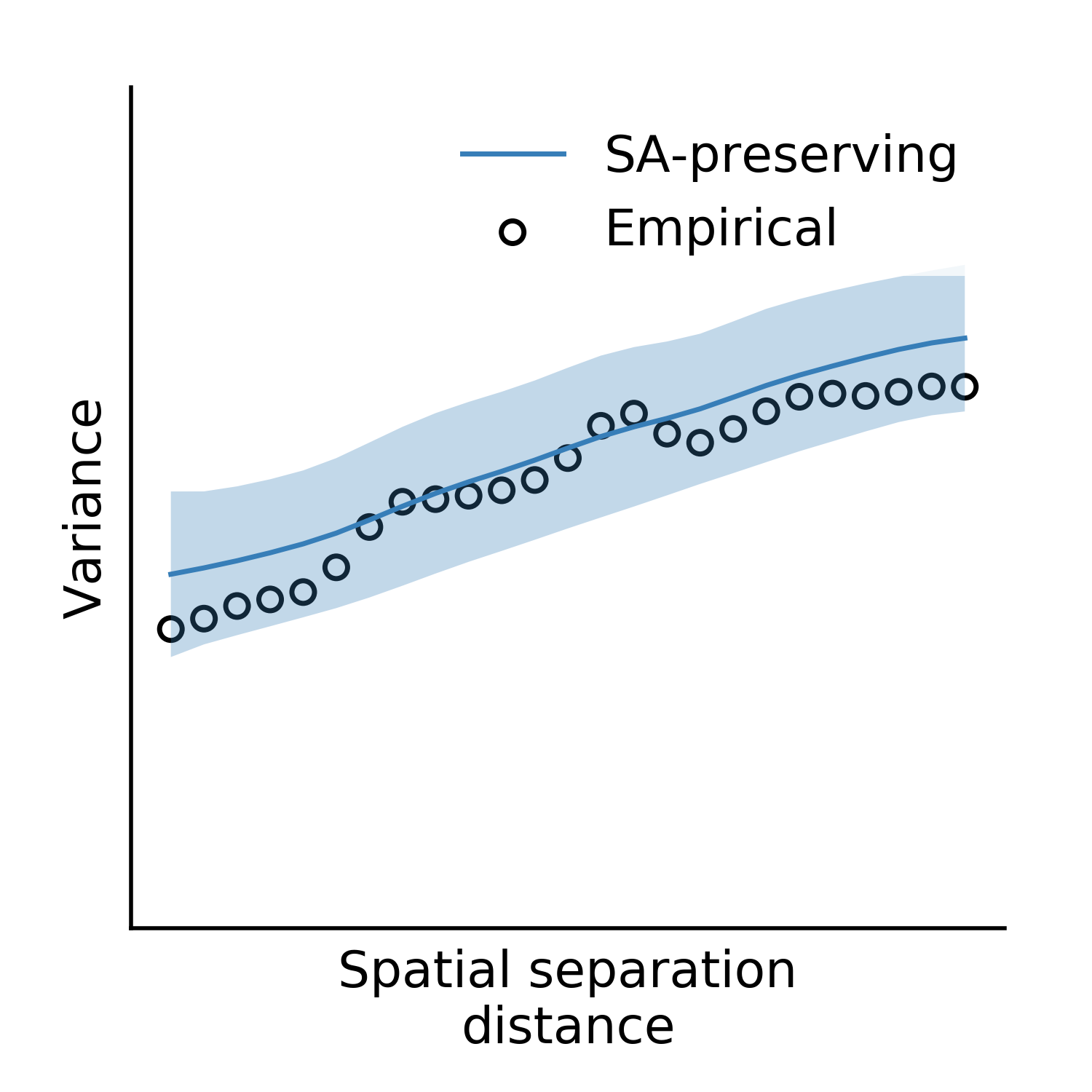
The surrogate maps exhibit the same autocorrelation structure as the empirical brain map.
Finally, we’ll compute non-parametric p-values using our two different null distributions:
from brainsmash.mapgen.stats import nonparp

print("Spatially naive p-value:", nonparp(test_stat, naive_brainmap_corrs))
print("SA-corrected p-value:", nonparp(test_stat, surrogate_brainmap_corrs))
The two p-values for this example come out to P < 0.001 and P=0.001, respectively.
Unilateral Subcortical Structure
For a subcortical analysis you’ll typically need:
A subcortical distance matrix
A subcortical brain map
A mask corresponding to a structure of interest
We’ll assume you use Connectome Workbench-style files and that you want to isolate one particular anatomical structure.
Note
If you already have a distance matrix and a brain map for your subcortical structure of interest, the workflow is identical to the cortical examples in Getting Started.
If you haven’t already computed a subcortical distance matrix or downloaded our pre-computed version, please follow these steps.
To isolate one subcortical structure from a whole-brain dscalar file, first do:
wb_command -cifti-export-dense-mapping yourfile.dscalar.nii COLUMN -volume-all output.txt -structure
We can then use the information contained in this file to isolate one particular structure, e.g. the left cerebellum:
from brainsmash.utils.dataio import load
import numpy as np
import pandas as pd

# Input files
image = "/path/to/yourfile.dscalar.nii"
wb_output = "output.txt"

# Load the output of the above command
df = pd.read_table(wb_output, header=None, index_col=0, sep=' ',
         names=['structure', 'mni_i', 'mni_j', 'mni_k']).rename_axis('index')

# Get indices for left cerebellum
indices = df[df['structure'] == 'CEREBELLUM_LEFT'].index.values

# Create a binary mask
mask = np.ones(31870)  # volume has 31870 CIFTI indices in standard 91k mesh
indices -= 59412  # first 59412 indices in whole-brain maps are cortical
mask[indices] = 0
np.savetxt("mask.txt", mask)  # this mask has right dimension for distmat

# Also saved a masked copy of the image
image_data = load(image)
indices += 59412  # assuming image data is whole-brain!
masked_image = image_data[indices]
np.savetxt("masked_image.txt", masked_image)
Next, we’ll need to sort and memory-map our distance matrix, but only for the pairwise distances between left cerebellar voxels:
from brainsmash.mapgen.memmap import txt2memmap

# Input files
image = "masked_image.txt"
mask = "mask.txt"
distmat = "/path/to/SubcortexDenseEuclideanDistmat.txt"

output_files = txt2memmap(distmat, output_dir=".", maskfile=mask, delimiter=' ')
Now, we can use the output files to instantiate our surrogate map generator. Here, we’ll also use the keyword arguments which were used in our study for left cerebellum. First, we’ll validate the variogram fit using these parameters:
from brainsmash.mapgen.eval import sampled_fit

x = "masked_image.txt"
distmat = output_files['distmat']
index = output_files['index']

kwargs = {'ns': 500,
          'knn': 1500,
          'nh': 25,
          'deltas': [0.3, 0.5, 0.7, 0.9],
          'pv': 70
          }

sampled_fit(x, distmat, index, nsurr=20, **kwargs)
This produces the following plot:
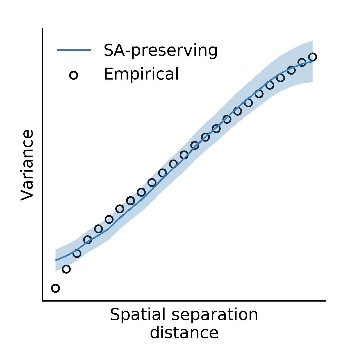
Having confirmed that the fit looks good, we simulate cerebellar surrogate maps with a call to the surrogate map generator:
from brainsmash.mapgen.sampled import Sampled

gen = Sampled(x, distmat, index, **kwargs)
surrogate_maps = gen(n=100)
Whole-Brain Volume
For this analysis you will need:
A text file containing voxel coordinates (with shape N rows by 3 columns)
A text file containing N brain map values
Your favorite neuroimaging software should be able to generate these files (e.g., AFNI).
Note
Do not include every voxel in the volume, but rather the voxels corresponding to your region of interest (e.g., the brain).
First, you will need to generate memory-mapped distance matrix files. This is
achieved using brainsmash.workbench.geo.volume, as in the code below:
from brainsmash.workbench.geo import volume

coord_file = "/path/to/voxel_coordinates.txt"
output_dir = "/some/directory/"

filenames = volume(coord_file, output_dir)
A dictionary containing the names of the newly generated files is returned by the function, which are used in the example below. Prior to generating surrogate maps, we first visually inspect the variogram fit:
from brainsmash.mapgen.eval import sampled_fit

brain_map = "/some_path_to/brain_map.txt"

# These are three of the key parameters affecting the variogram fit
kwargs = {'ns': 500,
          'knn': 1500,
          'pv': 70
          }

# Running this command will generate a matplotlib figure
sampled_fit(brain_map, filenames['D'], filenames['index'], nsurr=10, **kwargs)
If you are unhappy with the fit, it is recommended that you try varying the three
parameters included in the keyword argument dictionary above (i.e., ns, knn, and pv).
Note
A few users have reported a systematic overestimation of variance in their surrogate maps’ variograms. This suggests that further parameter tuning is necessary. However, it may also indicate a violation of the underlying assumption of stationary, which is more likely to be violated at the whole-brain level than within a single contiguous brain structure.
Having selected our parameter values and stored them in the kwargs dictionary,
we can now randomly generate surrogate brain maps with spatial autocorrelation that is matched to our target brain map:
from brainsmash.mapgen.sampled import Sampled

gen = Sampled(x=brain_map, D=filenames['D'], index=filenames['index'], **kwargs)
surrogate_maps = gen(n=1000)
These surrogate maps can then be used to test the null hypothesis that any random yet spatially autocorrelated brain map would yield a comparable or more extreme statistical result.