Getting Started

Input data types

Using BrainSMASH requires specifying two inputs:

• A brain map, i.e. a one-dimensional scalar vector, and

• A distance matrix, containing a measure of distance between each pair of elements in the brain map

For illustration’s sake, we will assume both required arguments have been written to disk as whitespace-separated text files LeftParcelMyelin.txt and LeftParcelGeodesicDistmat.txt. However, BrainSMASH can flexibly accommodate a variety of input types:

• Delimited *.txt files

• Neuroimaging files used by Connectome Workbench, including *scalar.nii files and *.func.gii metric files (assuming the files contain only a single brain map)

• Data and memory-mapped arrays written to *.npy files

• Numpy arrays and array-like objects

To follow along with the examples below, you can download our example data. Connectome Workbench users who wish to derive a distance matrix from a *.surf.gii file may want to begin below, as these functions take a long time to run (but thankfully only ever need to be run once).

Parcellated surrogate maps

For this example, we’ll make the additional assumption that LeftParcelMyelin.txt contains myelin map values for 180 unilateral cortical parcels, and that LeftParcelGeodesicDistmat.txt is a 180x180 matrix containing the pairwise geodesic distances between parcels.

Because working with parcellated data is not computationally expensive, we’ll import the brainsmash.mapgen.base.Base class (which does not utilize random sampling):

from brainsmash.mapgen.base import Base
brain_map_file = "LeftParcelMyelin.txt"  # use absolute paths if necessary!
dist_mat_file = "LeftParcelGeodesicDistmat.txt"

Note that if the two text files are not in the current directory, you’ll need to include the absolute paths to the files in the variables defined above.

We’ll create an instance of the class, passing our two files as arguments (implicitly using the default values for the optional keyword arguments):

base = Base(x=brain_map_file, D=dist_mat_file)

Surrogate maps can then be generated with a call to the class instance:

surrogates = base(n=1000)

where surrogates is a numpy array with shape (1000,180). The empirical brain map and one of the surrogate maps are illustrated side-by-side below for comparison:

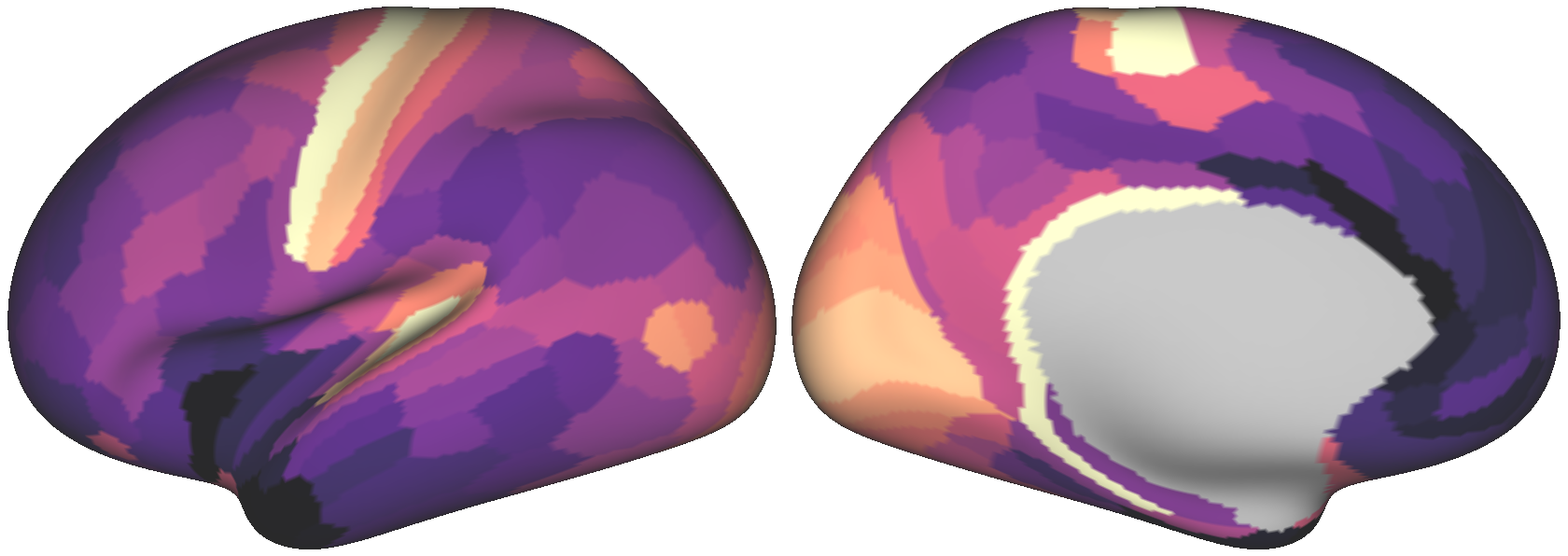
Fig. 3 The empirical T1w/T2w map.

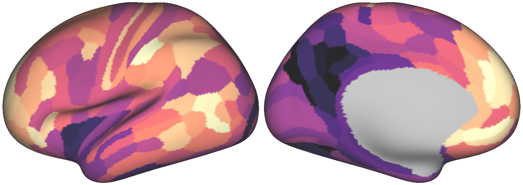
Fig. 4 One randomly generated surrogate map.

By construction, both maps exhibit the same degree of spatial autocorrelation in their values. However, notice that the empirical brain map has a distribution of values more skewed towards higher values, indicated by dark purple. If you wish to generate surrogate maps which preserve (identically) the distribution of values in the empirical map, use the keyword argument resample when instantiating the class:

base = Base(x=brain_map_file, D=dist_mat_file, resample=True)

The surrogate map illustrated above, had it been generated using resample=True, is shown below for comparison:

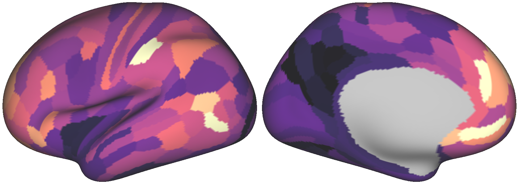
Fig. 5 The surrogate brain map above, with values resampled from the empirical map.

Note that using resample=True will in general reduce the degree to which the surrogate maps’ autocorrelation matches the autocorrelation in the empirical map. However, this discrepancy tends to be small for parcellated brain maps, and tends to be larger for brain maps whose values are more strongly non-normal.

Note

Shameless plug: the plots above were auto-generated using our wbplot package, available through both pip and GitHub. wbplot currently only supports cortical data, and parcellated data must be in the HCP’s MMP parcellation.

Keyword arguments to brainsmash.mapgen.base.Base

deltas np.ndarray or list[float], default [0.1,0.2,..,0.9]

The proportion of neighbors to include during the smoothing step, in the interval (0, 1]. This parameter specifies the different smoothing neighborhood sizes which are iterated over during the variogram optimization.

kernel str, default ‘exp’

The functional form of the smoothing kernel:

• ’gaussian’ : Gaussian function

• ‘exp’ : Exponential decay function

• ‘invdist’ : Inverse distance

• ‘uniform’ : Uniform weights (distance independent)

pv int, default 25

Percentile of the pairwise distance distribution at which to truncate during variogram fitting. The inclusion of this parameter is motivated by the fact that at large distances, pairwise variability is primarily driven by noise.

nh int, default 25

The number of uniformly spaced distance intervals within which to compute variance when constructing variograms. This parameter governs the granularity of your variogram. For noisy brain maps, this parameter should be small enough such that the variogram is smooth and continuous.

resample bool, default False

Resample surrogate maps’ values from empirical brain map, to preserve the distribution of values in each surrogate map. This may produce surrogate maps with poorer fits to the empirical map’s variogram.

b float or None, default None

The bandwidth of the Gaussian kernel used to smooth the variogram. The variogram isn’t particularly sensitive to this parameter, but it’s included anyways. If this parameter is None, by default the bandwidth is set to three times the variogram distance interval (see nh above).

Dense surrogate maps

Next, we’ll demonstrate how to use BrainSMASH to generate surrogate maps for dense (i.e., vertex- or voxel-wise) empirical brain maps, which is a little more tricky. Dense-level data are problematic because of their memory burden — a pairwise distance matrix for data in standard 32k resolution requires more than 4GB of memory if read in all at once from file.

To circumvent these memory issues, we’ve developed a second core implementation which utilizes memory-mapped arrays and random sampling to avoid loading all of the data into memory at once. However, users with sufficient memory resources and/or supercomputer access are encouraged to use the Base implementation described above.

Again, we’ll assume that the user already has a brain map and distance matrix saved locally as text files (or downloaded from here). Update as of Nov. 24, 2020: Per many requests from the community, BrainSMASH now includes functionality for users working with volumetric data at the whole-brain level. For details, please see the whole-brain volumetric example.

Creating memory-mapped arrays

Prior to simulating surrogate maps, you’ll need to convert the distance matrix to a memory-mapped binary file, which can be easily achieved in the following way:

from brainsmash.mapgen.memmap import txt2memmap
dist_mat_fin = "LeftDenseGeodesicDistmat.txt"  # input text file
output_dir = "."  # directory to which output binaries are written
output_files = txt2memmap(dist_mat_fin, output_dir, maskfile=None, delimiter=' ')

The latter two keyword arguments are shown using their default values. If your text files are comma-delimited, for example, use delimiter=',' instead. Moreover, if you wish to use only a subset of all brain regions, you may also specify a mask (as a path to a neuroimaging file) using the maskfile argument.

The return value output_files in the code block above is a dict type object that will look something like:

output_files = {'distmat': '/pathto/output_dir/distmat.npy',
                'index': '/pathto/output_dir/index.npy'}

These two files are required inputs to the brainsmash.mapgen.sampled.Sampled class.

Note

For additional computational speed-up, distmat.npy is sorted by brainsmash.mapgen.memmap.txt2memmap before it is written to file; the second file, index.npy, is required because it contains the indices which were used to sort the distance matrix.

This text to memory-mapped array conversion only ever needs to be run once for a given distance matrix.

Finally, to generate surrogate maps, we import the brainsmash.mapgen.sampled.Sampled class and create an instance by passing our brain map, memory-mapped distance matrix, and memory-mapped index file as arguments:

from brainsmash.mapgen.sampled import Sampled
brain_map_file = "LeftDenseMyelin.txt"  # use absolute paths if necessary!
dist_mat_mmap = output_files['distmat']
index_mmap = output_files['index']
sampled = Sampled(brain_map_file, dist_mat_mmap, index_mmap)

We then randomly generate surrogate maps with a call to the class instance:

surrogates = sampled(n=10)

Here, as above, we’ve implicitly left all keyword arguments – one of which is resample – left as their default values. The three images analogous to those shown above, illustrating the dense maps on the cortical surface, are shown below:

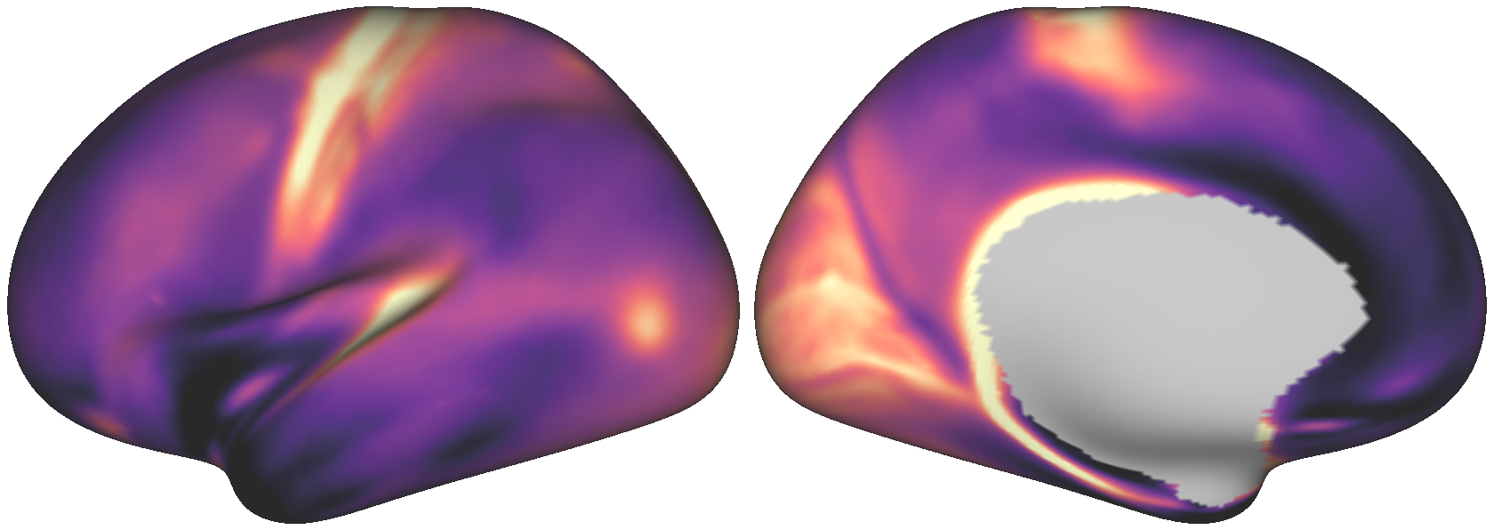
Fig. 6 The dense empirical T1w/T2w map.

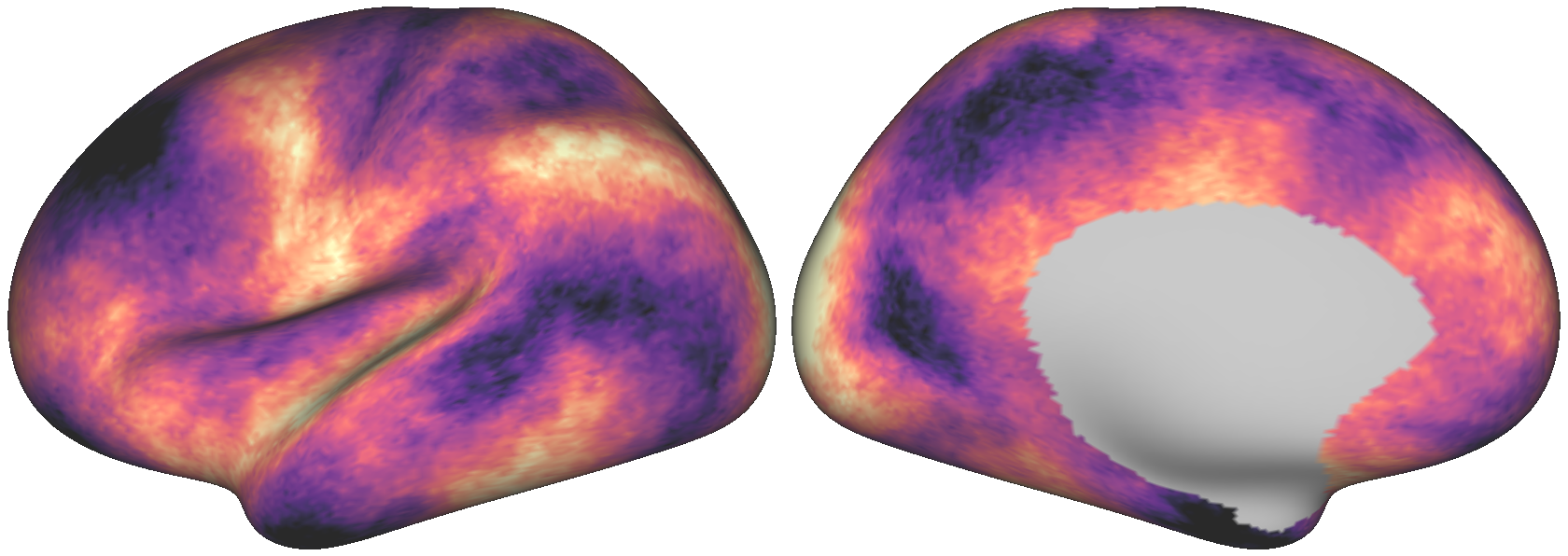
Fig. 7 One randomly generated dense surrogate brain map.

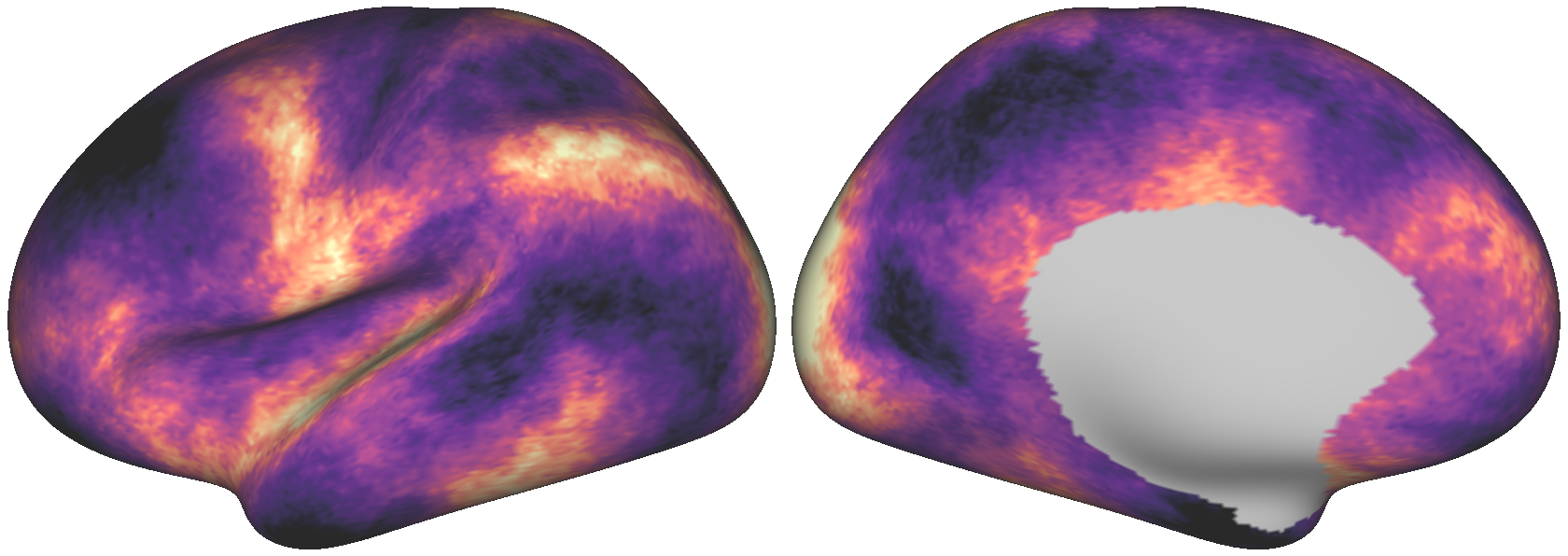
Fig. 8 The dense surrogate brain map above, with values resampled from the empirical map.

Keyword arguments to brainsmash.mapgen.sampled.Sampled

ns int, default 500

The number of randomly sampled brain areas used to generate a surrogate map.

knn int, default 1000

Let D be the pairwise distance matrix. Assume each row of D has been sorted, in ascending order. Then, because spatial autocorrelation is primarily a local effect, use only D[:,:knn].

deltas np.ndarray or list[float], default [0.3,0.5,0.7,0.9]

See above. Note that fewer values are iterated over by default than in the Base class. Users with more time and/or patience are encouraged to expand the default list, as it may improve your surrogate maps.

kernel str, default ‘exp’

See above.

pv int, default 70

See above. Note that this parameter is by default larger than for the Base class; this is in part because of the knn parameter above (which is used internally to reduce the distance matrix prior to determining pv.

nh int, default 25

See above.

resample bool, default False

See above.

b float or None, default None

See above.

Note

Dense data may be used with brainsmash.mapgen.base.Base – the examples are primarily partitioned in this way for illustration (but also in anticipation of users’ local memory constraints).

In general, the Sampled class has much more parameter sensitivity. You may need to adjust these parameters to get reliable variogram fits. However, you may use the functions in the variogram evaluation module, which we turn to next, to validate your variogram fits.

Evaluating variogram fits

To assess the reliability of your surrogate maps, BrainSMASH includes functionality to compare surrogate maps’ variograms to the target brain map’s variogram:

from brainsmash.mapgen.eval import base_fit
# from brainsmash.utils.eval import sampled_fit  analogous function for Sampled class
base_fit(brain_map_file, dist_mat_file, nsurr=100)

For well-chosen parameters, the code above will produce a plot that looks something like:

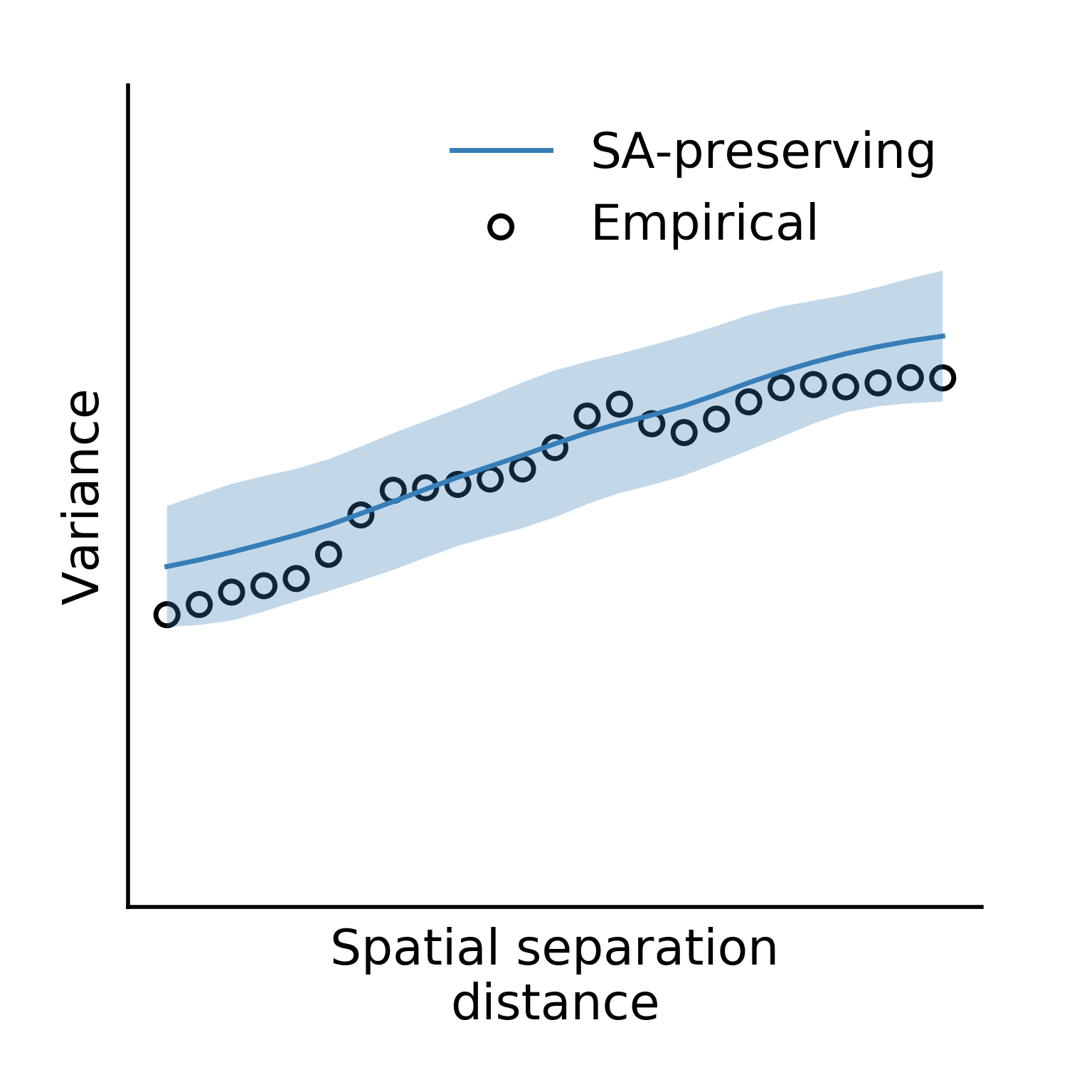
Fig. 9 Assessing the surrogate maps’ fit to the empirical data.

Shown above is the mean and standard deviation across 100 surrogates. Optional keyword arguments to the base and sampled class can be passed in the calls to the respective evaluation functions – for example, if you want to assess how changing model parameters influences your surrogates maps’ variogram fits.

Note

When using brainsmash.mapgen.eval.sampled_fit, you must specify the memory-mapped index file in addition to the brain map and distance matrix files (see above).

Workbench users

The functionality described below is intended for users using GIFTI- and CIFTI-format surface-based neuroimaging files.

Neuroimaging data I/O

To load data from a neuroimaging file into Python, you may use brainsmash.utils.dataio.load. For example:

from brainsmash.utils.dataio import load
objective = "/path/to/myimage.dscalar.nii"
x = load(objective)  # type(x) == numpy.ndarray

Computing a cortical distance matrix

To construct a geodesic distance matrix for a cortical hemisphere, you can do the following:

from brainsmash.workbench.geo import cortex
surface = "/path/to/S1200.L.midthickness_MSMAll.32k_fs_LR.surf.gii"
cortex(surface=surface, outfile="/pathto/LeftDenseGeodesicDistmat.txt", euclid=False)

Note that this function takes approximately two hours to run for standard 32k surface meshes. To compute 3D Euclidean distances instead of surface-based geodesic distances, simply pass euclid=True.

To compute a parcellated geodesic distance matrix, you could then do:

from brainsmash.workbench.geo import parcellate
infile = "/path/to/LeftDenseGeodesicDistmat.txt"
outfile = "/path/to/LeftParcelGeodesicDistmat.txt"
dlabel = "Q1-Q6_RelatedValidation210.CorticalAreas_dil_Final_Final_Areas_Group_Colors.32k_fs_L.dlabel.nii"
parcellate(infile, dlabel, outfile)

This code takes half an hour or less to run for the HCP MMP1.0. Note that the number of elements in dlabel must equal the number of rows/columns of your distance matrix. If you had a whole-brain parcellation file and needed to isolate the left cortical hemisphere, for example, you could do:

wb_command -cifti-separate yourparcellation_LR.dlabel.nii COLUMN -label CORTEX_LEFT yourparcellation_L.label.gii

You will then need to convert this GIFTI file to a CIFTI file:

wb_command -cifti-create-label yourparcellation_L.dlabel.nii -left-label yourparcellation_L.label.gii

For more information, see the -cifti-separate and -cifti-create-label documentation.

Computing a subcortical distance matrix

To compute a Euclidean distance matrix for subcortex, you could do the following:

from brainsmash.workbench.geo import subcortex
image_file = "/path/to/image_with_subcortical_volumes.dscalar.nii"
subcortex(outfile="/path/to/SubcortexDenseEuclidDistmat.txt", image_file=image_file)

Only three-dimensional Euclidean distance is currently implemented for subcortex. If you wish to create surrogate maps for a single subcortical structure, you can either generate your own mask file and pass it to brainsmash.mapgen.memmap.txt2memmap, or follow the procedure described here.

Note

If you mask your distance matrix, don’t forget to mask your brain map as well. One way this can be achieved is using brainsmash.workbench.io.image2txt.